• Simulated data is used everywhere in research to compare methods, models, algorithms, techniques etc. Simrel can be a common tool for such purpose

• Simulate linear model data with wide range of properties using small set of tuning paramters, Example:

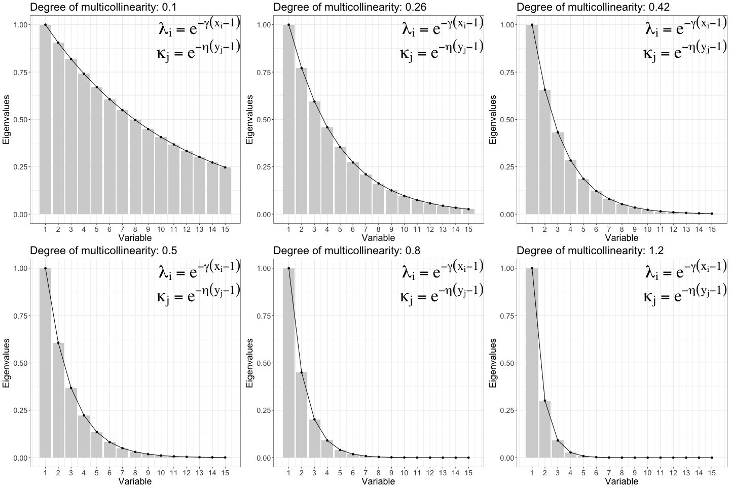
  • Controlling degree of multicollinearity in the simulated data

  • Specifying the relevant principle components for prediction

Reduction of regression Model: A Predictor sub-space ( blue) is relevant for informative response sub-space ( green). The idea discussed in 1 was implemented for single response in 2.

The Model:

\[\begin{bmatrix}y \\ x \end{bmatrix} \sim \text{N}\left( \begin{bmatrix} \mu_y \\ \mu_x \end{bmatrix}, \begin{bmatrix} \Sigma_{yy} & \Sigma_{yx}\\ \Sigma_{xy} & \Sigma_{xx} \end{bmatrix} \right)\]

Define a linear tranformation as \(z = Rx\) and \(w = Qy\), for any orthogonormal matrix \(R\) and \(Q\), we can imagine them as a rotation (eigenvector) matrix, so,

\[\begin{bmatrix}y \\ x \end{bmatrix} \sim \text{N}\left( \begin{bmatrix} Q^t\mu_w \\ R^t\mu_z \end{bmatrix}, \begin{bmatrix} Q^t\Sigma_{ww}Q & Q^t\Sigma_{wz}R\\ R^t\Sigma_{zw}Q & R^t\Sigma_{zz}R \end{bmatrix} \right)\]

There are \(\frac{1}{2}(p + m)(p + m + 1)\) unknowns to identify this model. But, …

Reduction of regression Model: A Predictor sub-space ( blue) is relevant for informative response sub-space ( green). The idea discussed in 1 was implemented for single response in 2.

\[ \begin{aligned} \Sigma_{ww} &= \text{diag}(\kappa_1, \ldots, \kappa_m), \kappa_j = e^{-\eta(y_j - 1), \; \eta > 0} \\ \Sigma_{zz} &= \text{diag}(\lambda_1, \ldots, \lambda_p), \lambda_i = e^{-\gamma(x_i - 1), \; \gamma > 0} \end{aligned} \]

We need to meet the constrains of coefficient of determinatin:

\[ \begin{aligned} \rho_w^2 &= \Sigma_{ww}^{-1/2} \Sigma_{zw}^{t} \Sigma_{zz}^{-1} \Sigma_{zw} \Sigma_{ww}^{-1/2} \\ \left(\rho_w^2\right)_{ij} &= \frac{\sigma_{ij}^t \Lambda ^{-1} \sigma_{ij'}}{\sqrt{\sigma_j^2\sigma_{j'}^2}} \forall j, j' = 1 \ldots m \end{aligned} \]

We assume there are no overlapping relevant components and there exist a subspace in predictor relevant to a subspace in response. This gives us,

\[ \rho_{w_j}^2 = \sum_{i=1}^p{\frac{\sigma^2_{ij}}{\lambda_i\kappa_j}} = \sum_{i\in \mathcal{P}}{\frac{\sigma^2_{ij}}{\lambda_i\kappa_j}} \]

Terminology:

• The informative response space is spanned by informative response components
• The relevant predictor space is spanned by relevant predictor components

sobj <- simrel(
  n = 20, p = 10, m = 4,
  q = c(5, 4),
  ypos = list(c(1, 4), c(2, 3)),
  relpos = list(c(1, 2), c(3, 5)), 
  R2 = c(0.8, 0.8),
  gamma = 0.6, eta = 0.2,
  type = "multivariate"
)

\[ \begin{aligned} \rho_{w_1}^2 &= \sum_{i\in \mathcal{P}}{\frac{\sigma^2_{i1}}{\lambda_i\kappa_1}}\\ &= \frac{\sigma_{11}^2}{\lambda_1\kappa_1} + \frac{\sigma_{21}^2}{\lambda_2\kappa_1} \end{aligned} \]

\[ \Sigma = \begin{bmatrix} \Sigma_{yy} & \Sigma_{yx}\\ \Sigma_{xy} & \Sigma_{xx} \end{bmatrix} \\ = \begin{bmatrix} Q^t\Sigma_{ww}Q & Q^t\Sigma_{wz}R\\ R^t\Sigma_{zw}Q & R^t\Sigma_{zz}R \end{bmatrix} \]

Define, \[\underset{n\times(m+p)}{G} = U\Sigma^{-1/2}\] \[\text{such that, } \text{cov}(G) = \Sigma\]

\[ \begin{aligned} \rho_{w_1}^2 &= \sum_{i\in \mathcal{P}}{\frac{\sigma^2_{i1}}{\lambda_i\kappa_1}}\\ &= \frac{\sigma_{11}^2}{\lambda_1\kappa_1} + \frac{\sigma_{21}^2}{\lambda_2\kappa_1} \end{aligned} \]

\[ \Sigma = \begin{bmatrix} \Sigma_{yy} & \Sigma_{yx}\\ \Sigma_{xy} & \Sigma_{xx} \end{bmatrix} \\ = \begin{bmatrix} Q^t\Sigma_{ww}Q & Q^t\Sigma_{wz}R\\ R^t\Sigma_{zw}Q & R^t\Sigma_{zz}R \end{bmatrix} \]

Define, \[\underset{n\times(m+p)}{G} = U\Sigma^{-1/2}\] \[\text{such that, } \text{cov}(G) = \Sigma\]

Relevant predictors has non-zero coefficients

Predictor components 3 and 5 (with low eigenvalues) are relevant to response component \(W_2\)

The properties propagate to related response variables

Education